Understanding the Empirical Rule Calculator: Your Gateway to Statistical Analysis
An empirical rule calculator is a powerful statistical tool that helps you quickly determine what percentage of your data falls within specific ranges of the mean. This calculator applies the famous 68-95-99.7 rule to analyze normally distributed datasets in seconds.
Quick Answer for Empirical Rule Calculator Users:
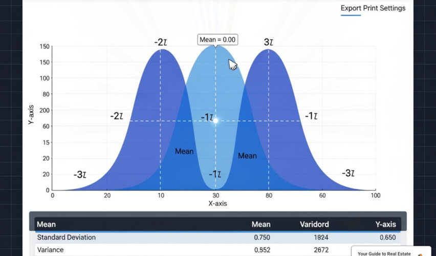
- 68% of data falls within 1 standard deviation of the mean
- 95% of data falls within 2 standard deviations of the mean
- 99.7% of data falls within 3 standard deviations of the mean
- Input required: Mean and standard deviation of your dataset
- Best for: Bell-shaped, normally distributed data
- Common uses: Real estate pricing analysis, quality control, identifying outliers
Whether you’re analyzing home prices in a neighborhood, examining test scores, or checking quality control data, the empirical rule calculator transforms complex statistical analysis into simple, actionable insights.
The tool eliminates manual calculations and reduces errors while helping you understand where your data points fall within the bigger picture. For real estate professionals, this means quickly identifying whether a property price is typical for the market or represents an outlier worth investigating.
The empirical rule is also known as the three-sigma rule because it covers three standard deviations from the mean, capturing nearly all data in a normal distribution.
, 95% within 2 standard deviations (middle sections), and 99.7% within 3 standard deviations (outer sections), with clear percentage labels and standard deviation markers - empirical rule calculator infographic")
What is the Empirical Rule (The 68-95-99.7 Rule)?
Picture this: you’re looking at home prices across different neighborhoods, and you’re drowning in a sea of numbers. How do you make sense of it all? That’s exactly where the Empirical Rule becomes your best friend in data analysis.
The Empirical Rule, also called the 68-95-99.7 rule or the three-sigma rule, is like having a statistical roadmap for understanding your data. It tells you exactly how information spreads around the average in a normal distribution – that classic bell-shaped curve you’ve probably seen before.
Here’s what makes this rule so powerful: it works with any normally distributed data, whether you’re analyzing home prices, test scores, or quality control measurements. The beauty lies in its simplicity – you only need to know the mean (average) and standard deviation to open up valuable insights about your entire dataset.
Think of the standard deviation as a measuring stick that shows how spread out your data is from the average. When your data forms that perfect symmetrical bell curve, the Empirical Rule becomes incredibly reliable for predicting outcomes and understanding data spread.
For a deeper understanding of these concepts, you can explore more about Understanding the Empirical Rule and how professionals apply it in real-world scenarios.
The Three Core Principles
The magic of the Empirical Rule comes down to three memorable percentages that work like clockwork with normally distributed data:
68% of your data lives within 1 standard deviation of the mean. This is your core data zone. If average home prices in a neighborhood are $300,000 with a standard deviation of $20,000, then 68% of homes sold between $280,000 and $320,000.
95% of your data falls within 2 standard deviations of the mean. This captures the vast majority of your information. Using our home price example, 95% of properties would sell between $260,000 and $340,000. This range gives you excellent insight into typical market behavior.
99.7% of your data sits within 3 standard deviations of the mean. This encompasses almost everything – we’re talking about 99.7% of all data points falling between $240,000 and $360,000 in our real estate scenario. Anything outside this range? Those are rare outliers worth investigating.
These percentages aren’t random – they’re mathematical constants that appear consistently in normal distributions. This reliability makes the empirical rule calculator such a valuable tool for quick analysis.
Why It Only Applies to Normally Distributed Data
Here’s the catch: the Empirical Rule is picky about the data it works with. It only applies to normally distributed data – information that forms that perfect, symmetrical bell curve.

A normal distribution has specific bell curve characteristics: it’s perfectly symmetrical around the mean, has a single peak, and tapers off evenly on both sides. This symmetry around the mean is crucial because the rule’s percentages depend on this balanced distribution.
When your data is skewed (leans heavily to one side) or has multiple peaks, the 68-95-99.7 percentages simply don’t hold true anymore. Imagine a neighborhood with mostly modest homes but a few multi-million dollar mansions – that data would be positively skewed, making the Empirical Rule unreliable.
This is why checking for normality is essential before applying the rule. You need that classic bell shape for accurate predicting outcomes. Understanding when to use the rule – and when not to – is just as important as knowing how to use it.
For more detailed information about normal distributions and their properties, check out this comprehensive guide on normal distribution to ensure you’re applying statistical tools correctly.
How to Use an Empirical Rule Calculator Step-by-Step
Learning to use an empirical rule calculator is like finding a shortcut that saves you hours of tedious math. Whether you’re analyzing property values in your neighborhood or checking quality control data for your business, this tool transforms complex statistical analysis into something anyone can master in minutes.

Most online calculators feature a clean, simple interface that won’t intimidate you. You’ll typically see two main input fields: one for the mean (μ) and another for the standard deviation (σ) of your dataset. Some advanced calculators even accept raw data directly, automatically crunching the numbers for you behind the scenes.
The process is refreshingly straightforward. First, you’ll gather your data – perhaps a list of recent home sales in your target area or monthly rental prices for similar properties. Next, you need to calculate the mean by adding up all values and dividing by the total count. Then comes the standard deviation, which measures how spread out your data points are from that average.
Once you have these two key numbers, simply input them into the calculator and hit that calculate button. Within seconds, you’ll see the ranges for one, two, and three standard deviations from the mean, complete with the percentage of data expected to fall within each range.
Why Use an Empirical Rule Calculator?
Time is precious, especially when you’re making important financial decisions about real estate investments. An empirical rule calculator delivers several game-changing advantages that make it indispensable for modern data analysis.
Speed and efficiency top the list – what used to take 15-20 minutes of careful calculation now happens instantly. You can analyze multiple datasets in the time it once took to process just one. This rapid analysis is crucial when you’re evaluating properties in a competitive market where opportunities disappear quickly.
Avoiding manual errors becomes equally important as your datasets grow larger. Even math whizzes make mistakes when juggling multiple calculations, and a single error can throw off your entire analysis. Calculators eliminate this risk entirely, giving you confidence in your results.
The tool provides instant data range calculation for all three standard deviation levels simultaneously. Instead of performing separate calculations for 68%, 95%, and 99.7% ranges, you get everything at once. This comprehensive view helps you understand the full picture of your data distribution.
For analyzing large datasets – imagine processing hundreds of property sales or rental listings – manual calculation becomes practically impossible. The calculator makes this feasible and efficient, allowing you to spot trends and opportunities that might otherwise remain hidden. This capability proves especially valuable when applying Marketing Fundamentals to understand market segments and customer behavior patterns.
Manual Calculation: The Formula Explained
While the empirical rule calculator handles the heavy lifting beautifully, understanding the underlying formulas gives you deeper insight into what’s actually happening with your data. Think of it as learning to read the map even when you have GPS – sometimes you need to understand the route.
The process starts with calculating the mean (μ), which is simply your data’s average. Add up all your values and divide by the total count: μ = (Σ xi) / n. This gives you the center point around which everything else revolves.
Standard deviation calculation gets a bit more involved, and here’s where it matters whether you’re working with a complete population or just a sample. For a population standard deviation, you use: σ = √ [ (Σ (xi – μ)²) / n ]. For a sample standard deviation, the formula becomes: s = √ [ (Σ (xi – x̄)²) / (n – 1) ]. Notice that crucial (n-1) in the sample formula – this adjustment helps provide a more accurate estimate when you’re working with incomplete data.
Once you have both the mean and standard deviation, applying the rule becomes straightforward. 68% of your data falls within μ ± 1σ, 95% falls within μ ± 2σ, and 99.7% falls within μ ± 3σ. These ranges give you powerful insight into what’s normal versus what’s unusual in your dataset.
For deeper exploration of practical applications, Employing the Empirical Rule in Statistical Problems offers excellent worked examples that bring these concepts to life.
Interpreting Results from an Empirical Rule Calculator
The magic happens when you translate those calculator results into real-world insights. Let’s say you’re analyzing monthly rental prices for two-bedroom apartments in your city, and your calculator shows a mean of $1,500 with a standard deviation of $100.
Your results would show three key ranges: $1,400 to $1,600 captures about 68% of typical rents, $1,300 to $1,700 encompasses 95% of the market, and $1,200 to $1,800 includes virtually all properties at 99.7%. These ranges function like confidence intervals, helping you understand probability and likelihood.
When a new apartment lists for $1,850, you immediately recognize it as an outlier – priced above 99.7% of similar properties. This could signal either exceptional value (luxury finishes, prime location) or overpricing. Conversely, finding a unit at $1,150 suggests either a great deal or potential issues worth investigating.
Making predictions becomes much easier with this framework. You can confidently tell clients that most two-bedroom apartments in the area rent between $1,300 and $1,700, while anything outside $1,200 to $1,800 represents unusual market conditions.
Identifying where specific data points fall within these ranges helps assess risk and opportunity. A property priced in the 68% range represents typical market conditions, while those in the outer ranges warrant closer examination. This systematic approach to data interpretation proves invaluable whether you’re applying Stock Market Terminology to investment analysis or evaluating real estate opportunities for long-term growth potential.
Real-World Applications: From Test Scores to Real Estate
The beauty of the empirical rule calculator lies in how it transforms abstract statistics into practical, everyday solutions. You’ll find this powerful tool working behind the scenes in countless industries, helping professionals make smarter decisions with their data.

Think about a teacher grading standardized tests. If the average score is 75 with a standard deviation of 8 points, she immediately knows that 68% of her students scored between 67 and 83. Any student scoring below 59 or above 91 (outside two standard deviations) deserves special attention—either for extra help or advanced placement.
Manufacturing companies rely on this rule for quality control. When producing car parts, they know that 99.7% of properly manufactured components will fall within three standard deviations of the target measurement. Anything outside that range gets flagged for inspection.
Finance professionals use the empirical rule to assess investment risk. If a stock’s monthly returns average 2% with a standard deviation of 4%, they can predict that 95% of the time, monthly returns will fall between -6% and +10%. This helps investors set realistic expectations and manage their portfolios.
Even IQ scores follow this pattern perfectly. With an average of 100 and standard deviation of 15, we know that 68% of people score between 85 and 115, while scores above 130 or below 70 represent just 5% of the population.
Analyzing Real Estate Market Data
Here’s where the empirical rule calculator becomes your secret weapon in real estate analysis. Instead of drowning in spreadsheets of property prices, you can quickly understand market patterns and spot opportunities.
Let’s walk through a real example from a neighborhood analysis. Imagine you’re studying home prices in a suburban area where the mean home price sits at $425,000 with a standard deviation of $65,000.
Your empirical rule calculator reveals that 68% of homes sell between $360,000 and $490,000—this is your bread-and-butter market range. When clients ask about “typical” prices, you have a confident, data-backed answer.
95% of properties fall between $295,000 and $555,000, representing the vast majority of sales. This broader range helps you understand the full scope of the local market.
The 99.7% range spans from $230,000 to $620,000. Properties outside this range are statistical rarities that deserve special attention.
This analysis transforms how you approach market stability. A neighborhood with a small standard deviation suggests consistent, predictable pricing—great for conservative investors. A larger standard deviation might indicate a diverse market with various property types and price points, offering more opportunities for different buyer segments.
When identifying undervalued or overvalued properties, the empirical rule becomes invaluable. A $650,000 listing immediately stands out as potentially overpriced or uniquely valuable. Similarly, a $220,000 property might represent an incredible deal or signal underlying issues worth investigating.
This statistical approach gives you the confidence to guide clients through How to Invest in Real Estate decisions with solid data backing your recommendations.
Using the Rule to Identify Outliers
One of the most exciting applications of the empirical rule is its ability to flag unusual data points that demand your attention. Since 99.7% of normally distributed data falls within three standard deviations, anything outside this range represents less than 0.3% of all observations—making it statistically extraordinary.
These outliers tell fascinating stories. Sometimes they reveal data entry errors—like when a $4,250,000 listing appears in your $425,000 neighborhood analysis because someone added an extra zero. Quick outlier detection saves you from embarrassing mistakes in client presentations.
More often, outliers represent exceptional circumstances worth investigating. That $650,000 home in our example might feature stunning architectural details, waterfront access, or recent luxury renovations that justify its premium price. Understanding what makes properties exceptional helps you better serve clients looking for unique features.
On the flip side, unusually low-priced properties often signal opportunities or challenges. A $200,000 home in a $425,000 neighborhood might be a foreclosure, need major repairs, or have other factors affecting its value. These findies can lead to excellent investment opportunities for the right buyer.
Outlier analysis also reveals market trends and helps with Real Estate Business Growth strategies. If you notice more high-end outliers appearing over time, it might signal neighborhood gentrification or increasing demand for luxury features.
The key is treating outliers as conversation starters rather than data mistakes. Each unusual data point has a story, and understanding these stories makes you a more knowledgeable, effective real estate professional.
Understanding the Rule’s Limitations
Every great tool has its boundaries, and the empirical rule calculator is no exception. While it’s incredibly useful for analyzing data, it’s not magic—it won’t work correctly in every situation. Think of it like a specialized wrench that’s perfect for certain bolts but useless on others.
The biggest limitation is that the Empirical Rule only works with normally distributed data. Beautiful bell curve we talked about? Your data needs to look like that for the 68-95-99.7 percentages to be accurate. If your data doesn’t follow this pattern, using the rule is like trying to steer with the wrong map—you’ll end up in the wrong place.
Here’s when you should avoid using the Empirical Rule:
When your data is skewed, meaning it leans heavily to one side rather than being symmetrical. Real estate markets sometimes show this pattern—most homes might be modestly priced, but a few luxury properties create a long tail of high prices.
If you’re dealing with bimodal distributions, where your data has two distinct peaks instead of one. Imagine analyzing home prices in an area with both affordable starter homes and expensive luxury properties, creating two separate clusters.
With small sample sizes, it’s tough to know if your data truly follows a normal distribution. You need a decent amount of data to see the bell curve pattern clearly.
For more insights on this fundamental concept, you can explore our detailed guide on the Empirical Rule.
What to Do with Non-Normally Distributed Data
Don’t panic if your data doesn’t fit that perfect bell curve! You’re not stuck without options. This is where Chebyshev’s Inequality becomes your backup plan—it’s like having a reliable friend who’s always there when your first choice falls through.
Chebyshev’s theorem is much more flexible than the Empirical Rule. It works with any distribution shape—skewed, flat, bumpy, you name it. The catch? It gives you less precise estimates. Instead of telling you exactly what percentage of data falls within certain ranges, it gives you minimum guarantees.
Here’s how they compare:
| Feature | Empirical Rule | Chebyshev’s Inequality |
|---|---|---|
| Data Requirements | Must be bell-shaped (normal) | Works with any shape |
| Precision | Exact percentages (68%, 95%, 99.7%) | Minimum percentages only |
| Within 2 Standard Deviations | Exactly 95% of data | At least 75% of data |
| Within 3 Standard Deviations | Exactly 99.7% of data | At least 88.9% of data |
Think of it this way: the Empirical Rule is like a precise GPS that only works on paved roads, while Chebyshev’s Inequality is like a compass that works anywhere but gives you a general direction rather than exact coordinates.
When you’re analyzing real estate data that doesn’t follow a normal pattern, Chebyshev’s theorem still helps you understand your data spread. It won’t be as precise as your empirical rule calculator, but it’s better than flying blind. You’ll know that at least 75% of your property values fall within two standard deviations of the average, even if the exact percentage might be higher.
Frequently Asked Questions about the Empirical Rule Calculator
When people start using an empirical rule calculator for the first time, they often have similar questions. Let me walk you through the most common ones to help clear up any confusion and make you more confident in using this powerful statistical tool.
What is the difference between using the empirical rule for sample vs. population data?
This is one of the most important distinctions to understand, and honestly, it trips up a lot of people at first. The good news is that the 68-95-99.7 percentages stay exactly the same whether you’re working with a sample or an entire population. The difference lies in how you calculate the standard deviation that goes into your empirical rule calculator.
When you have population data (like every single home sale in a city for the entire year), you use the population standard deviation formula with ‘n’ in the denominator. But here’s the thing—most of the time in real estate, we’re working with sample data. Maybe you’re looking at a selection of recent sales or homes in a particular price range.
For sample data, you need to use the sample standard deviation formula, which has (n-1) in the denominator instead of just ‘n’. This small change is called Bessel’s correction, and it’s there because samples naturally tend to underestimate how spread out the full population really is. Think of it as a statistical safety net that gives you a more honest picture.
The impact on your results can be meaningful. Using the wrong formula might give you standard deviation values that are too small, which would make your data ranges too narrow. Most quality empirical rule calculators will ask you to specify whether you’re working with sample or population data, so pay attention to that choice.
Can the empirical rule be used to prove a dataset is normal?
I get this question a lot, and the short answer is no, it can’t prove normality. But don’t worry—it’s still incredibly useful as a quick check or guideline to see if your data might be normally distributed.
Think of the empirical rule as a helpful screening tool. If your data closely follows the 68-95-99.7 pattern, that’s a great sign that you’re probably dealing with a normal distribution. But it’s more like a first impression than a final verdict.
For definitive proof, you’d need to use formal statistical tests like the Shapiro-Wilk test or create visual inspections with histograms. But for most practical purposes in real estate analysis, if your data behaves according to the empirical rule, you’re usually safe to proceed.
Here’s a practical way to think about it: if you’re analyzing home prices in a neighborhood and they follow the expected percentages pretty closely, you can confidently use the empirical rule for your analysis. If the numbers seem way off, that’s when you might want to dig deeper into whether the data is actually normally distributed.
How accurate is the 68-95-99.7 rule?
The empirical rule gives you remarkably accurate approximations for normally distributed data, but it’s important to understand that it’s based on a theoretical, perfectly symmetrical normal distribution. Real-world data is rarely perfect, and that’s completely normal (no pun intended).
In practice, you might find that 67% or 69% of your data falls within one standard deviation instead of exactly 68%. Or maybe 94% or 96% falls within two standard deviations rather than precisely 95%. These small variations are totally acceptable and don’t diminish the rule’s usefulness.
The beauty of the empirical rule lies in its reliability as a rule of thumb. It’s been used successfully across countless industries and applications because it consistently provides excellent estimations for approximately normal data. When you’re making quick decisions about property values or market trends, these approximations are more than accurate enough to guide your choices.
For real estate professionals, this level of accuracy is particularly valuable because it allows you to quickly assess whether a property price is typical for the market or represents an outlier worth investigating further. The slight variations from the exact percentages don’t change the practical insights you’ll gain from using an empirical rule calculator.
Conclusion
What a journey we’ve taken together through statistical analysis! We started with a simple question—how can we quickly understand data spread?—and finded that the answer lies in the neat simplicity of the empirical rule calculator and its famous 68-95-99.7 percentages.
Think about where you were when we began this exploration. Perhaps statistics felt intimidating, or maybe you weren’t sure how data analysis could help in real estate decisions. Now you’re equipped with a powerful tool that transforms complex datasets into clear, actionable insights in just minutes.
The beauty of the Empirical Rule lies in its accessibility. You don’t need a statistics degree to understand that 68% of normally distributed data falls within one standard deviation of the mean. You don’t need advanced mathematical training to recognize that a property priced three standard deviations above the neighborhood average deserves a closer look. The empirical rule calculator puts this power directly in your hands.
For real estate professionals and investors, this knowledge is particularly valuable. Whether you’re analyzing home prices in Dallas, rental rates in Oklahoma City, or market trends across different neighborhoods, the ability to quickly identify typical ranges and spot outliers gives you a significant advantage. It’s the difference between making gut-feeling decisions and making informed, data-driven choices.
Remember the key takeaways we’ve covered: The rule works beautifully for bell-shaped, normally distributed data. It helps you understand where most of your data lives and quickly identifies the unusual cases that might represent opportunities or red flags. When your data isn’t normally distributed, tools like Chebyshev’s Inequality can step in to help.
Most importantly, this statistical tool aligns perfectly with our mission at Your Guide to Real Estate—providing you with proven frameworks and stress-free guidance for success. When you can quickly analyze market data and understand property valuations relative to their neighborhoods, you’re making decisions from a position of strength rather than uncertainty.
The next time you encounter a dataset, whether it’s property values, rental yields, or market trends, you’ll know exactly what to do. Fire up an empirical rule calculator, input your mean and standard deviation, and let the 68-95-99.7 rule reveal the story hidden in your numbers.
That’s the real power of statistical literacy—changing raw information into the insights that drive successful real estate decisions.
Get expert guidance on valuation and market analysis in real estate.
Connect with Us:
Follow Us On: Facebook
Follow Us On: LinkedIn
Follow Us On: Twitter
Follow Us On: YouTube


")